Lab 7: Analyzing proportions

Estimate population proportions and their uncertainty using confidence intervals, and conduct hypothesis tests on proportions.

Learning Objectives

By the end of this lab, students will be able to:

  • Explain how measures of center (mean, median) and spread (SD, SE) summarize different aspects of a distribution
  • Explain how mean and median differ in skewed distributions and describe how each summarizes the data
  • Create and interpret summary tables of grouped data using descriptive statistics
  • Explain the difference between SD and SE in words, and describe what each does and does not represent
  • Use the 2SE rule of thumb to describe uncertainty in group means, without making inferential claims
  • Interpret different graph types used to address distributional versus mean-based questions
  • Describe patterns in data clearly using both figures and concise Results-style text

Getting started

Before you begin the lab activities, review the steps for setting up a project for a lab activity:

Then, complete the following steps to make sure you are fully set up.

  1. Get the Lab Worksheet.

    Pick up a physical copy of the lab worksheet, or print one if you are working outside of class.
    Download Lab Worksheet (PDF, if needed)

  2. Open Posit Cloud and start Lab 7.

  3. Install required packages

    • tidyverse

    • palmerpenguins

    • lterdatasampler

  4. Create an R Script

  5. Load the packages

NoteCheckpoint

At this point, you should have:

  • These instructions open in a web browser.
  • Your Lab 7 project open in Posit Cloud in another browser window.
  • The required packages installed and loaded without errors
  • The Lab 7 worksheet in front of you.

Do not continue until all of the above steps are working correctly.

Overview

In this lab you will learn how to work with proportions (a special case of a mean when the variable is binary).

You will practice four closely related tasks:

  1. Estimate a proportion (e.g., the proportion of females in a sample).
  2. Quantify uncertainty in that estimate using a 95% confidence interval (CI).
  3. Test a hypothesis about a population proportion, such as whether the true proportion is 0.5.
  4. Visualize the estimated proportions and their confidence intervals.

Conceptually:

  • A sample proportion is an estimate of a population proportion.
  • A confidence interval gives a plausible range of values for the population proportion, based on your sample.
  • A hypothesis test evaluates whether your data are consistent with a specific claim (e.g., p = 0.5).

In R, you can do both the CI and hypothesis test with the same function: prop.test().

Worked example: penguin sex ratio (proportions, CI, and a hypothesis test)

In this worked example, we will use the penguins dataset to:

  • Estimate the proportion of penguins that are female and male (based on non-missing sex)
  • Calculate a 95% CI for the proportion that are female
  • Test the hypothesis that the population proportion of females is p = 0.5

Example R code

# Load packages ----

library(tidyverse)
library(palmerpenguins)


# Import and clean dataset ----

penguins_clean <-
  penguins |> 
  filter(!is.na(sex))


# Analysis ----

penguins_summary <- 
  penguins_clean |>
  summarize(
    n_sex = n(),
    .by = sex
  ) |> 
  mutate(
    n_total = sum(n_sex),
    p_hat = n_sex / n_total,
    se = sqrt(p_hat * (1 - p_hat) / n_total),
    p_prime = (n_sex + 2) / (n_total + 4),
    ci_lower = p_prime - 1.96 * sqrt(p_prime * (1 - p_prime) / (n_total + 4)),
    ci_upper = p_prime + 1.96 * sqrt(p_prime * (1 - p_prime) / (n_total + 4))
  ) |> 
  print()
# A tibble: 2 × 8
  sex    n_sex n_total p_hat     se p_prime ci_lower ci_upper
  <fct>  <int>   <int> <dbl>  <dbl>   <dbl>    <dbl>    <dbl>
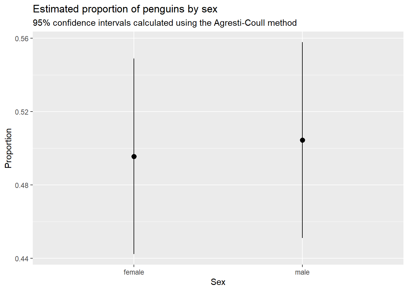
1 male     168     333 0.505 0.0274   0.504    0.451    0.558
2 female   165     333 0.495 0.0274   0.496    0.442    0.549
# Graph estimates and CIs ----

ggplot(penguins_summary) +
  geom_pointrange(aes(x = sex, y = p_hat, ymin = ci_lower, ymax = ci_upper)) +
  labs(
    x = "Sex",
    y = "Proportion",
    title = "Estimated proportion of penguins by sex",
    subtitle = "95% confidence intervals calculated using the Agresti-Coull method"
  )

# Hypothesis test ----

n_female <- 
  penguins_summary |> 
  filter(sex == "female") |> 
  pull(n_sex)

n_total <-
  penguins_summary |> 
  filter(sex == "female") |> 
  pull(n_total)

prop.test(x = n_female, n = n_total, p = 0.5, correct = FALSE)

    1-sample proportions test without continuity correction

data:  n_female out of n_total, null probability 0.5
X-squared = 0.027027, df = 1, p-value = 0.8694
alternative hypothesis: true p is not equal to 0.5
95 percent confidence interval:
 0.4421534 0.5489403
sample estimates:
        p 
0.4954955 

Interpreting the output (what you should be able to say)

After running the code, you should be able to report:

  • The estimated proportion female (your point estimate)

  • The 95% CI for the proportion female

  • The p-value for the test of p = 0.5, and whether you would reject at a typical alpha level (e.g., 0.05)

  • Keep the interpretation strictly about the population proportion of females and whether the data are consistent with 0.5.

Student task: repeat the workflow with bison sex

In this task, you will apply the same workflow to the knz_bison dataset from the lterdatasampler package, using animal_sex.

The knz_bison dataset

This dataset contains records of American bison sampled at Konza Prairie. For this lab you will focus on:

  • animal_sex (a categorical variable)

Your tasks

Using bison with non-missing animal_sex:

  1. Create a frequency table of animal_sex and report the sample size used.

  2. Estimate the proportion female (and the proportion male, if present).

  3. Compute a 95% CI for the proportion female using prop.test().

  4. Conduct a hypothesis test of H0: p_female = 0.5 (two-sided) using prop.test().

  5. Write 2–4 sentences summarizing your results in plain language, including:

    • the sample size for each sex

    • your estimate of the proportion female the 95% CI

    • the p-value and a clear conclusion about whether the data support p = 0.5

Wrap-up and submission

Before leaving lab:

  1. Make sure your R script is saved in your Posit Cloud project and runs from top to bottom without errors.

  2. Verify you have completed the student task (estimate, CI, hypothesis test, and answer questions on worksheet).

  3. Show your worksheet, graph, and R script to an LA to get completion credit for the lab.