Lab 2: Workflow and Data Types

Working with data frames in R using the palmerpenguins dataset to practice data inspection, data types, and simple summaries.

Student Learning Outcomes

By the end of lab you should be able to:

Access our Posit Cloud workspace and start a project from a template.
Load course packages (the tidyverse) and access the palmerpenguins dataset.
Inspect a dataset to answer:
- How many observations/variables?
- What are the variable names?
- What are their data types?
Produce quick summaries of all variables.
Explore the relationship between two numerical variables using a scatterplot.

Important

Paper handout: You will answer questions on a paper worksheet as you move through this page. This page will tell you exactly when to answer each question (e.g., Worksheet Q1).

Download Lab Worksheet (PDF, if needed)

Setup and workflow

1) Join the course workspace on Posit Cloud

Open the course Posit Cloud link from the D2L announcement.
Sign in with your Posit Cloud account.
Join the course workspace. You will be redirected to a Welcome screen.

Worksheet Q1

Write down the name of the workspace you joined. You can see this in the left navigation bar under Spaces.

Tip

If you are already in the workspace, proceed to the next step.

2) Start your Lab 2 project from the template

In the course workspace, click the Content heading to see projects in the workspace.
Click the bluen START button the Lab 2 project. This will create your own copy of the project and open it.

Worksheet Q2:

What is the name of your Lab 2 project?

Note

Why we use Projects: Projects keep your code, data, and outputs together in one folder and make relative file paths work reliably.

3) Create an R script

In your Lab 2 project, create a new R script:

In the Files pane, click New File → R Script.
Save the file immediately.
Name the script: lab-02.R

Packages and the penguins dataset

4) Packages for this course

In R, shared code is distributed as packages (bundles of functions, data, and documentation).
In this course we will use the tidyverse in every lab moving forward.

For this lab you will use:

tidyverse (especially dplyr, ggplot2, readr, tibble)
palmerpenguins (the dataset source)

Install packages

Copy the code from the box below by clicking the clipboard icon, paste it into the Console (not your script), and run it to install the required packages.

install.packages(c("tidyverse", "palmerpenguins"))

Load packages (run every new session)

Put this at the top of your script and run it:

# load packages -----------------------------------------------------------

library(tidyverse)      # tools for working with data
library(palmerpenguins) # penguin dataset

Worksheet Q3:

What is the difference between installing a package and loading a package?

tidyverse messages

When you load the tidyverse, you will see some messages in the console. These are telling you that tidyverse is loading some other packages for you, and that some of their functions have the same name as some functions in base R packages.

You can usually just ignore these messages.

Data frames, tibbles, and penguins

5) What is a data frame? What is a tibble?

A data frame is the basic table-like data structure in R:

Rows = observations (cases, individuals, sampling units)
Columns = variables (measurements or categories)

A tibble is a modern version of a data frame used by the tidyverse:

Prints in a cleaner way (doesn’t flood your console)
Keeps variable types visible
Plays nicely with tidyverse functions

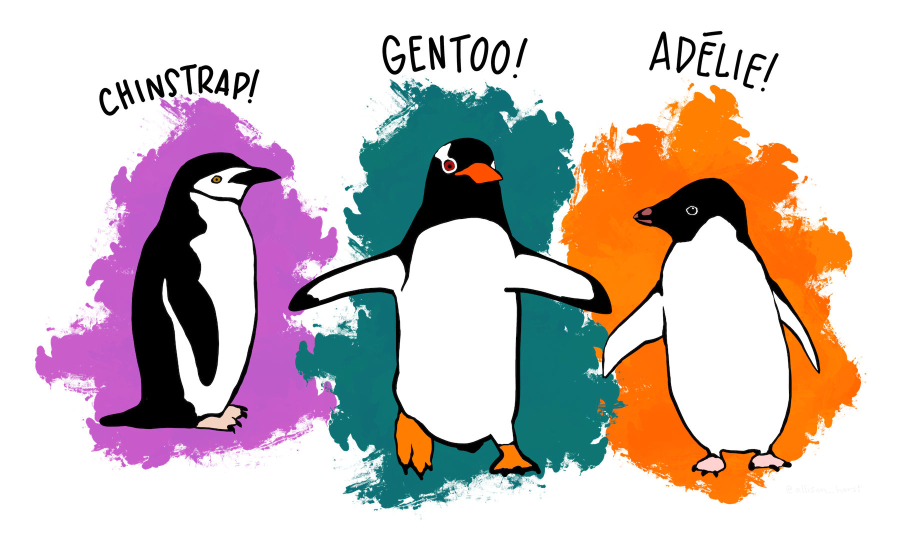
The palmerpenguins package includes a dataset named penguins with measurements from penguins in the Palmer Archipelago (Antarctica).

Illustrated image showing three penguins standing side by side against colorful paint-splash backgrounds, representing the three species in the palmerpenguins dataset: Chinstrap, Gentoo, and Adélie. — Stylized illustrations of the three penguin species in the *palmerpenguins* dataset—Chinstrap, Gentoo, and Adélie—commonly used for teaching data visualization and data analysis in R. Artwork by @allison_horst

Run this to print the penguins object in the console:

penguins

# A tibble: 344 × 8
   species island    bill_length_mm bill_depth_mm flipper_length_mm body_mass_g
   <fct>   <fct>              <dbl>         <dbl>             <int>       <int>
 1 Adelie  Torgersen           39.1          18.7               181        3750
 2 Adelie  Torgersen           39.5          17.4               186        3800
 3 Adelie  Torgersen           40.3          18                 195        3250
 4 Adelie  Torgersen           NA            NA                  NA          NA
 5 Adelie  Torgersen           36.7          19.3               193        3450
 6 Adelie  Torgersen           39.3          20.6               190        3650
 7 Adelie  Torgersen           38.9          17.8               181        3625
 8 Adelie  Torgersen           39.2          19.6               195        4675
 9 Adelie  Torgersen           34.1          18.1               193        3475
10 Adelie  Torgersen           42            20.2               190        4250
# ℹ 334 more rows
# ℹ 2 more variables: sex <fct>, year <int>

Worksheet Q4:

What does a row represent in the penguins dataset? What does a column represent?

Inspecting a dataset and identifying variable types

6) Basic inspection tools

There are many functions that give you information about a dataset. Some, like the next example, are basic functions included in R.

Size: `nrow()` and `ncol()`

The classic way to inspect a dataset is will functions like nrow() and ncol, which return the number of rows and columns in a data frame.

nrow(penguins)
ncol(penguins)

Worksheet Q5:

How many rows and columns are in penguins?

Print: look at a few rows (without printing everything)

With modern tibbles, printing in the console provides the same information as the previous two functions, plus a lot more.

Run the following lines of code, pausing to see the output after each line. Can you spot where the number of rows and columns is displayed in the output?

print(penguins)
print(penguins, n = 15, width = Inf)  # show more rows and all columns

Structure overview: `glimpse()`

This is the fastest way to see:

variable (column) names
variable types (R classes)
a preview of values

glimpse(penguins)

Rows: 344
Columns: 8
$ species           <fct> Adelie, Adelie, Adelie, Adelie, Adelie, Adelie, Adel…
$ island            <fct> Torgersen, Torgersen, Torgersen, Torgersen, Torgerse…
$ bill_length_mm    <dbl> 39.1, 39.5, 40.3, NA, 36.7, 39.3, 38.9, 39.2, 34.1, …
$ bill_depth_mm     <dbl> 18.7, 17.4, 18.0, NA, 19.3, 20.6, 17.8, 19.6, 18.1, …
$ flipper_length_mm <int> 181, 186, 195, NA, 193, 190, 181, 195, 193, 190, 186…
$ body_mass_g       <int> 3750, 3800, 3250, NA, 3450, 3650, 3625, 4675, 3475, …
$ sex               <fct> male, female, female, NA, female, male, female, male…
$ year              <int> 2007, 2007, 2007, 2007, 2007, 2007, 2007, 2007, 2007…

Worksheet Q6:

From glimpse(penguins), list three variables in the penguins dataset.

Quick counts: `dplyr::count()`

Use count() to see how many observations fall in each category:

count(penguins, species)
count(penguins, island)

Worksheet Q7:

Which species is most common in the dataset? How many rows are there for that species?

7) Connecting lecture data types to R variable types

In lecture, you learned data types like nominal, ordinal, discrete, and continuous.

In R, what you see in glimpse() is usually a class (type) such as:

character (text)
factor (categorical with a fixed set of levels)
logical (TRUE/FALSE)
integer (whole numbers)
double / numeric (numbers with decimals)

These two systems overlap, but they are not identical. This table is a practical crosswalk:

Lecture concept	Typical meaning	Common R type(s) you’ll see	Short name in a tibble	Notes
Nominal (categorical)	categories with no order	`factor`, `character`	`fct`, `chr`	`factor` is preferred for “known categories”
Ordinal (categorical)	categories with order	`factor` (ordered)	`fct`	ordering must be defined explicitly
Discrete (numeric)	counts (0, 1, 2, …)	`integer`, sometimes `double`	`int`	counts can be stored as numeric even if “discrete”
Continuous (numeric)	measured on a continuum	`double` / `numeric`	`dbl`	most measurements are `double`

Worksheet Q8:

Choose two variables in penguins and write their type using (a) lecture terminology and (b) R type from glimpse().

Summarizing variables

8) Summaries you can generate quickly

Base R summary: `summary()`

This gives different summaries depending on variable type:

summary(penguins)

For numeric variables: min, quartiles, median, mean, max (plus NAs)
For categorical variables: counts per category (plus NAs)

Worksheet Q9:

Use summary(penguins) to answer: Which variable(s) show missing values?

Thinking about relationships between variables

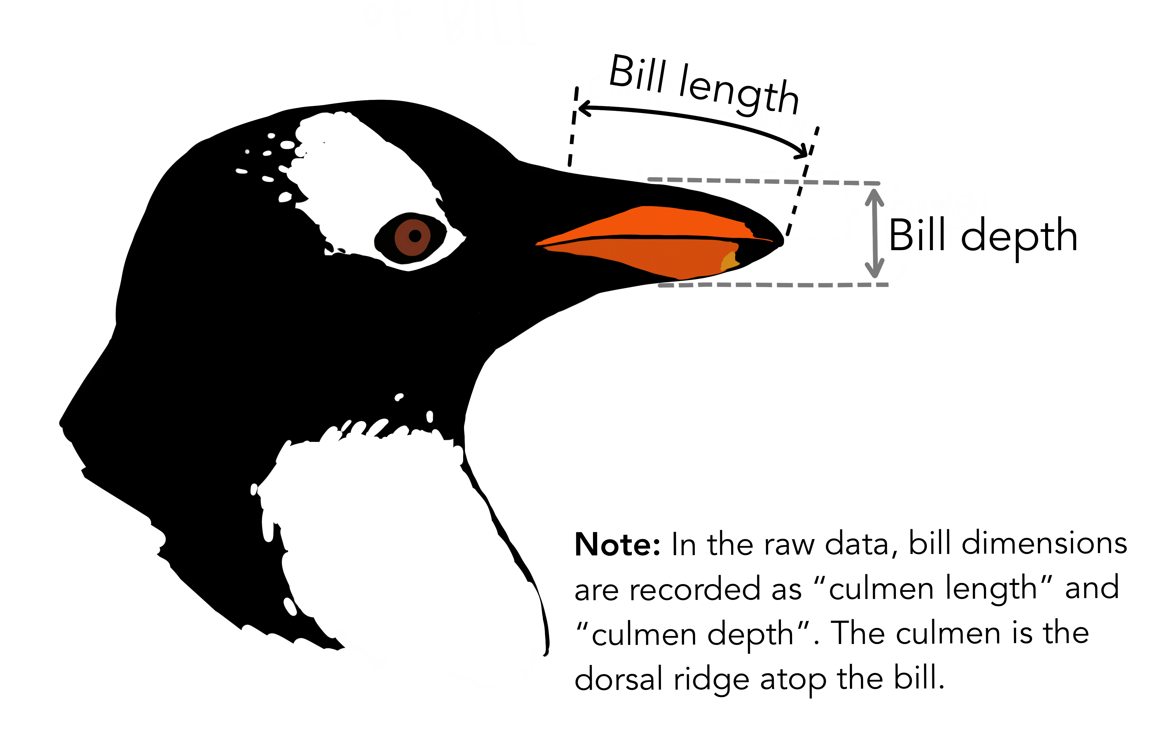
In this section, you will explore the relationship between two penguin traits: bill length and bill depth. These measurements describe different dimensions of the penguin’s bill and are commonly used to study variation among individuals and species. Refer to the diagram below to be clear on what is meant by length versus depth.

Labeled diagram of a penguin head showing two bill measurements: bill length measured along the top ridge of the bill from base to tip, and bill depth measured vertically at the base of the bill. — Diagram illustrating penguin bill (culmen) measurements, showing how bill length is measured along the ridge of the upper bill and bill depth is measured vertically at the base of the bill. Artwork by @allison_horst

9) Predict the relationship before plotting

Before running any code, think about how these two variables might be related. If a penguin has a longer bill, do you expect it to also have a deeper bill, or might there be little or no relationship between them?

Worksheet Q10

Sketch your prediction by:

Drawing x- and y-axes

Labeling the axes bill length and bill depth

Drawing a line or pattern that shows how you think the two variables are related

Do this before you generate the plot in R.

10) Make a scatterplot with ggplot2

The following code example is adapted from the palmerpenguins package website:
https://allisonhorst.github.io/palmerpenguins/articles/examples.html

Copy this code to your script exactly as written:

ggplot(
  data = penguins, 
  mapping = aes(x = bill_length_mm, y = bill_depth_mm, group = species)
) +
  geom_point(
    aes(color = species, shape = species),
    size = 3, 
    alpha = 0.8
  ) +
  geom_smooth(method = "lm", se = FALSE, aes(color = species)) +
  scale_color_manual(values = c("darkorange", "purple", "cyan4")) +
  labs(
    title = "Penguin bill dimensions",
    subtitle = "Bill length and depth for Adelie, Chinstrap and Gentoo Penguins at Palmer Station LTER",
    x = "Bill length (mm)",
    y = "Bill depth (mm)",
    color = "Penguin species",
    shape = "Penguin species"
  ) +
  theme(
    legend.position = c(0.85, 0.15),
    plot.title.position = "plot",
    plot.caption = element_text(hjust = 0, face = "italic"),
    plot.caption.position = "plot"
  )

Worksheet Q11:

Briefly interpret the plot:

What is the relationship between bill length and bill depth?

Do species appear to differ? How?

Wrap-up and submission

Make sure your script is saved in your Lab 2 project.
Keep your worksheet and show it to a Learning Assistant to have it initialed before you leave lab. You may do this as soon as you finish.

Student Learning Outcomes

Setup and workflow

1) Join the course workspace on Posit Cloud

2) Start your Lab 2 project from the template

3) Create an R script

Packages and the penguins dataset

4) Packages for this course

Install packages

Load packages (run every new session)

Data frames, tibbles, and penguins

5) What is a data frame? What is a tibble?

Inspecting a dataset and identifying variable types

6) Basic inspection tools

Size: nrow() and ncol()

Print: look at a few rows (without printing everything)

Structure overview: glimpse()

Quick counts: dplyr::count()

7) Connecting lecture data types to R variable types

Summarizing variables

8) Summaries you can generate quickly

Base R summary: summary()

Thinking about relationships between variables

9) Predict the relationship before plotting

10) Make a scatterplot with ggplot2

Wrap-up and submission

Size: `nrow()` and `ncol()`

Structure overview: `glimpse()`

Quick counts: `dplyr::count()`

Base R summary: `summary()`