install.packages("tidyverse")Lab 3: Importing Data into R
Reading external data into R using tidyverse tools, with emphasis on file structure, missing values, and verifying that imported data match the meaning of the original dataset.
Learning Objectives
By the end of this lab, you should be able to:
- Read a CSV file into R using
read_csv()and verify that it imported correctly. - Identify when default import settings are insufficient based on the structure of a data file.
- Recognize how missing values are represented in a dataset and how R interprets them.
- Manually set data types.
Getting Started
Before beginning the lab, make sure you are set up correctly.
Pick up a physical copy of the lab worksheet, or print one if you are working outside of class.
Download Lab Worksheet (PDF, if needed)Log in to Posit Cloud and navigate to the course workspace.
Open the Assignment Project named “Lab 3 Importing Data”
Install the required packages for this lab (tidyverse) using the Packages pane or by running the following code in the Console pane (do not put it in a script):
Create a new R script and save it as lab-3-script.R.
-
Copy and paste this code to the top of your script in the Source pane and run it to load the tidyverse package:
- The first line is a comment that RStudio recognizes as a section heading.
- The second line loads the tidyverse package so that you can use functions in it later.
WarningIf you run
library(tidyverse)before you install the tidyverse package, you will see an error message in the console like this:Error in library(tidyverse) : there is no package called tidyverseThe solution is to install the package first, then load it with
library().
Overview: Introduction to importing data
In this lab, you will learn how data are brought into R from an external file. Unlike the previous lab, where the dataset already existed in R, this lab focuses on what happens before analysis begins.
Reading data into R is not a passive step. When you import a dataset, R must make decisions about where the data begin, how missing values are represented, and how different variables should be interpreted. R provides reasonable defaults, but those defaults are guesses. It is your responsibility to check them and, when necessary, override them.
The goal of this lab is not to analyze data, make plots, or run statistical tests. The goal is to practice reading data correctly and verifying that the imported dataset matches the meaning of the original data source.
With the project set up and the required package loaded, we will begin by reading a CSV file that is already well-structured and works with R’s default assumptions.
Tip
Read the following sections carefully before writing any code or answering handout questions. The lab will clearly indicate when you should run code or record an answer. Skipping ahead often leads to confusion and unnecessary frustration.
CSV Files and the Project Environment
The datasets used in this lab are stored as CSV (comma-separated values) files. A CSV file is a plain text file where:
- each row represents an observation
- each column represents a variable
- values are separated by commas.
CSV files are widely used because they are simple, portable, and can be read by many different programs, including R.
All data files for this course are stored in a folder named data/ inside the project. This folder structure will be used consistently throughout the semester.
Before reading any data into R, take a moment to explore the project directory:
- Open the Files pane in RStudio
- Navigate into the
data/folder - Look for files with names that end in
.csv
The part of the file name after the final dot is called the file extension. Files that end in .csv are CSV files. For example:
-
example-data.csvis a CSV file -
example-data.xlsxis not a CSV file
In this course, file names will always:
- use hyphens (
-), not underscores (_) - be written entirely in lowercase
Handout Q1
List all CSV files you see in the
data/folder.
For each file, write its relative path, starting from the project root.A relative path includes the folder name(s) and the filename, separated by forward slashes.
Example format:
-data/example-data.csv(Include all CSV files currently present in the folder.)
When you are finished, return to the project’s top-level folder by clicking the .. entry in the Files pane. You can also click the R cube icon in the Files pane to return directly to the project root.
Caution
Seeing a file in the Files pane means it exists on disk, but it is not available in R until you read it using code. R does not automatically load files just because they are present in the project.
Read on to learn how to read data using R code.
Reading a CSV File with read_csv()
We will begin by reading a real epidemiological dataset using read_csv(). This provides a concrete example of what it looks like when a CSV file is already well-structured and can be read using R’s default assumptions.
Before writing any code, take a moment to read the dataset description below so you understand what the data represent.
WNV Dataset overview
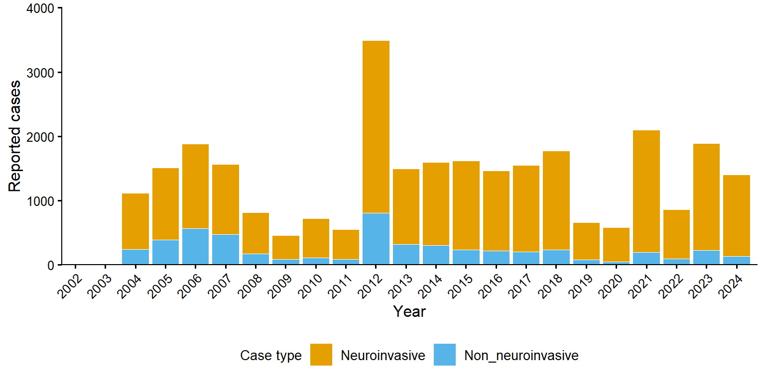
The file wnv-data.csv contains state-level West Nile virus hospitalization data from the Arbonet (here). The dataset is titled:
West Nile virus hospitalizations by case type and year of illness onset, 2004–2024
Study context:
This dataset summarizes reported hospitalizations associated with West Nile virus infection in the United States, broken down by year of illness onset and case type.
Unit of observation:
A single reporting year.
Variables:
-
year- the year of illness onset -
case_type- type of case: neuroinvasive or non-neuroinvasive -
reported_cases- number of cases reported
Inspect the CSV file before reading it into R
Before reading the dataset into R, take a moment to look at the file itself.
- Open the Files pane in RStudio on Posit Cloud
- Navigate to the
data/folder - Click on
wnv-data.csvto open it in the file viewer
Spend a minute inspecting the contents of the file directly. You are not running any code yet—this step is about understanding what R will be asked to interpret.
As you look at the file, consider the following questions:
- What are the variable (column) names?
- What type of data does each variable appear to contain (e.g., numeric counts, categorical labels)?
- Are there any missing values, and if so, how do they appear to be represented in the file?
Handout Q2
List the three variables and state whether they are nominal, ordinal, continuous, or numerical discrete.
Handout Q3
What value represents a missing value (no data) in this dataset?
Reading the file
Now that you know what the data file should contain (based on the dataset description and metadata), and what it does contain (based on your inspection of the CSV), you are ready to read it into R.
To read this dataset into R, use the read_csv() function. The only required argument is the path to the file, which you recorded in your answer to handout question 1.
The file is stored in the project’s data/ folder, so you must include that folder in the path name, for example data/wnv-data.csv. Here is example code to read a hypothetical `data/example.csv` data file:
# read the data ----------------------------------------------------------

read_csv("data/example.csv")
Important
The file path must be surrounded by double quotes `"`.
Copy and paste that code into your R script, then modify the path so it references the wnv-data.csv file instead of example.csv.
Running that line of code will cause R to read the data into a tibble in R and print that tibble in the console.
Inspect the console output to confirm:
- the variable names are correct,
- each column contains the expected type of data,
- and the number of rows matches the expected number of years.
Handout Q4
How many observations are there in the dataset?
While the previous code will read the data and print it in the console, it will not assign the dataset a name and make it available for further actions. To do that, you must use the assignment operator <- to give the tibble a name, for example:
wnv_data <- read_csv("data/wnv-data.csv")You can give the dataset any name you want. In this case we have named it wnv_data.
Now you can do other actions with the data, like glimpsing or summarizing it using functions learned in the previous lab. For example:
This example shows what it looks like when a CSV file aligns well with R’s defaults. In the next sections of the lab, you will work with datasets that require additional instructions—such as skipping non-data lines or explicitly defining missing values—to be read correctly.
Skipping Non-Data Lines
Many real datasets include information at the top of the file that is not part of the data table. These lines may describe the data source, reporting notes, or collection methods. R does not know which lines are metadata and which lines contain the actual data unless you tell it.
Drug Efficacy Trial Dataset
This dataset should be included in your Posit Cloud project, but you can also download it here:
Description
This dataset comes from a simulated clinical drug efficacy trial designed to resemble how data are recorded in FDA-style studies. Each row represents a single participant at a single study visit, so most participants appear multiple times in the dataset.
Participants were randomly assigned to one of three treatment arms—placebo, low dose, or high dose—and were measured at baseline and follow-up visits during the study. The outcome variable is a continuous biomarker value that is expected to change over time in response to treatment.
Some follow-up measurements are missing because participants did not complete every visit. In the raw data file, missing outcome values are recorded using an explicit text code rather than being left blank. Part of your task in this lab is to recognize how missing values are represented and ensure that R interprets them correctly when the data are read in.
Unit of observation
An individual study participant at a single study visit.
Variables
-
STUDYID- Identifier for the clinical study. All records in this dataset come from the same study. -
USUBJID- Unique participant identifier. Each participant has a single ID that appears on multiple rows corresponding to different study visits. -
SITEID- Identifier for the clinical site where the participant was enrolled. -
ARMCD- Short code identifying the treatment arm to which the participant was assigned (e.g., placebo, low dose, high dose). -
ARM- Human-readable label for the treatment arm. -
PARAMCD- Short code for the outcome being measured. -
PARAM- Description of the outcome variable measured in the study. -
AVISITN- Numeric visit identifier indicating the study time point (e.g., 0 = baseline, 4 = Week 4, 8 = Week 8). Although numeric, this variable represents discrete study visits, not a continuous time scale. -
AVISIT- Human-readable label for the study visit. -
BASE- Baseline value of the outcome variable for each participant. A continuous numerical variable. -
AVAL- Observed outcome value at the given visit. Missing follow-up values are recorded using a text codeNRin the raw data file. A continuous numerical variable.
Some variables appear redundant because clinical datasets often include both short codes and human-readable labels (e.g., treatment arm or visit) so that the same data can be used reliably for analysis while remaining clear and interpretable in tables and figures.
Inspect the CSV
Before reading the file into R, open the CSV itself to see what it contains.
- In the Files pane, navigate to the
data/folder. - Click on the CSV file you will be using for this section.
When the file opens, look carefully at the first few lines. You should notice that not every line contains actual data values. Some lines at the top of the file provide background information about the dataset rather than observations.
This is common in real datasets, especially those shared publicly or generated for reporting. These lines are useful for humans, but R does not know to ignore them unless you tell it to.
Handout Q5
Which line contains the variable names?
Handout Q6
How many lines of non-data before the first row of data? (should be one less than the previous answer).
The answer to the second question tells you how many lines you need to skip when reading the data file to import the data into R.
Read the file
Start by reading the file without any special arguments. This lets you see what happens when R treats every line as data.
trial_data <- read_csv("data/drug-trial-data.csv")After running this code, look at the output carefully. You may see:
- warnings about parsing problems
- The text
Columns: 1indicating only one column was read - Column names that do not look correct.
These issues are not mistakes on your part. They happen because R is trying to interpret non-data lines as if they were part of the table.
Print the object trial_data in the console (copy this to your script and run it):
trial_dataYou should see that the data is a tibble with 362 rows and 1 column named Simulated clinical trial dataset for BIOL 275 (NOT real patient data).
The first line of “data” contains Format: long; one record per participant per visit., while the third line of data contains the variable names.
Set the skip argument
To fix this, you need to tell R how many lines to skip at the top of the file before reading the actual data.
If the first two lines of the file contain descriptive text rather than column names, you can skip them using the skip argument.
trial_data <- read_csv("data/drug-trial-data.csv", skip = 2)Now print trial_data in the console again. It should look more like what you expected the first time.
Handout Q7
How many rows and columns are in the correctly-imported
trial_datatibble?
Setting missing values
Inspect the printed output of trial_data in the console.
Handout Q8
What data type does it show for the variable
AVAL? What data type should it be based on what the variable represents?
Next, run summary(trial_data) to see how R summarizes the variables when the missing values are still recorded as text.
You should notice that AVAL is currently listed as a character variable. This happens because the column includes the text value NR, which is being used in the file to indicate missing data. When a column contains any text values, R has no choice but to treat the entire column as character data.
To remind yourself what a properly recognized missing value looks like in R, print wnv_data in the console again and compare the output. Also look at summary(wnv_data) and compare the output to summary(trial_data).
Handout Q9
How do the
NAvalues inwnv_datadiffer from theNRvalues you see intrial_datawhen the file is first read?
To tell R that the text value NR should be treated as a missing value, you need to set the na argument when reading the file.
trial_data <- read_csv(
  "data/drug-trial-data.csv",
  skip = 2,
  na = "NR"
)

trial_data
After running this code, look closely at the printed output in the console. In particular, notice how the missing values are now displayed and how the data type of AVAL has changed.
Handout Q10
What data type is
AVALafter settingna = "NR"?
Defining levels of categorical variables
Character variables vs. factors
In R, categorical variables are often stored in one of two ways:
-
character (
chr) - plain text values (e.g.,"Baseline","Week 4","Week 8"). R treats these as labels, with no special structure. -
factor (
fct) - categorical values with a defined set of levels (and an optional meaningful order). Factors are designed for categorical data and are commonly used in statistical models.
You can usually make the same plots in ggplot using either chr or fct. However, factors give you better control over:
- the order of categories in axes and legends,
- how categories are handled in statistical models,
- and whether category order should be treated as meaningful (ordered factors).
Ordered vs. unordered factors
All factors have an internal ordering of their levels, but only ordered factors tell R that the order has meaning. This matters most for comparisons and for how variables are treated in statistical models.
Use:
- unordered factors for categories with no natural ranking (e.g., sites, states),
- ordered factors for categories with a meaningful progression (e.g., time points, dose levels).
| Aspect | Unordered factor | Ordered factor |
|---|---|---|
| Level order exists | Yes | Yes |
| Order has meaning | No | Yes |
< / > comparisons allowed |
No | Yes |
| Default model behavior | Nominal (separate groups) | Ordinal (trend-aware contrasts) |
| ggplot appearance | Usually the same | Usually the same |
Handout Q11
Which variables in the dataset, if any, should be treated as unordered factors? Which should be treated as ordered factors?
Example 1: Turning SITEID into an unordered factor
Before changing a variable, always inspect its values so you know what levels exist.
count(trial_data, SITEID)SITEID identifies enrollment sites. There is no meaningful ranking among sites, so this variable should be an unordered factor.
Example 2: Turning AVISIT into an ordered factor
Next, inspect the visit variable.
count(trial_data, AVISIT)These visits represent study time points (Baseline → Week 4 → Week 8). Even though they are discrete categories, their order reflects time and therefore has meaning.
Set the factor levels explicitly and mark the factor as ordered.
Read the bird dataset
Practice: Reading and Preparing a Bird Point Count Dataset
In this section, you will work with a new dataset and apply everything you have learned so far about importing data into R.
This bird point count dataset is intentionally structured to require the same decisions you have already practiced. Before writing any code, inspect the CSV file and think about what R will need in order to read it correctly.
As you work through this dataset, you should be prepared to:
- skip non-data lines at the top of the file,
- tell R how missing values are recorded,
- inspect variables to determine their appropriate data types,
- convert character variables to factors where appropriate,
- and decide whether any factors should be ordered.
You may refer back to earlier examples, but you should not need to learn any new functions for this section.
Bird Point Count Dataset overview
This dataset contains simulated results from point count surveys for birds. Each observation represents a bird species at a particular point at a given date and time.
-
point_ididentifies the survey point. -
speciesindicates which bird species was counted (Grasshopper Sparrow, Lark Sparrow, or Baltimore Oriole). -
datetimerecords the date and time of the survey visit. -
windis the wind level on the Beaufort scale (0–4), which is an ordinal categorical variable. -
bird_countis the number of birds detected (a count).
Instructions
Inspect the CSV dataset before reading it into R, converse with at leat two of your classmates, and answer the following questions:
Handout Q12
How many rows should you skip?
Handout Q13
Which column contains missing values, and what text represents a missing value?
Handout Q14
Which variables should be converted to nominal categorical variables? ordinal categorical variables?
Write the code to perform the necessary steps to read the data and set the categorical variable types.
Tip
Handout Q15
Print the final bird dataset in the console and show it to an LA for grading.
Wrap-up and submission
- Make sure your script is saved in your project on Posit Cloud.
- Print the final bird dataset in the console and show it to an LA for grading.
- Keep your handout and show it to a Learning Assistant for a completion grade before you leave lab. You may do this as soon as you finish.